Various utils
Flowpaths implements various helper functions on graphs. They can be access with the prefix flowpaths.utils.
Graph visualization and drawing
You can create drawing as this one
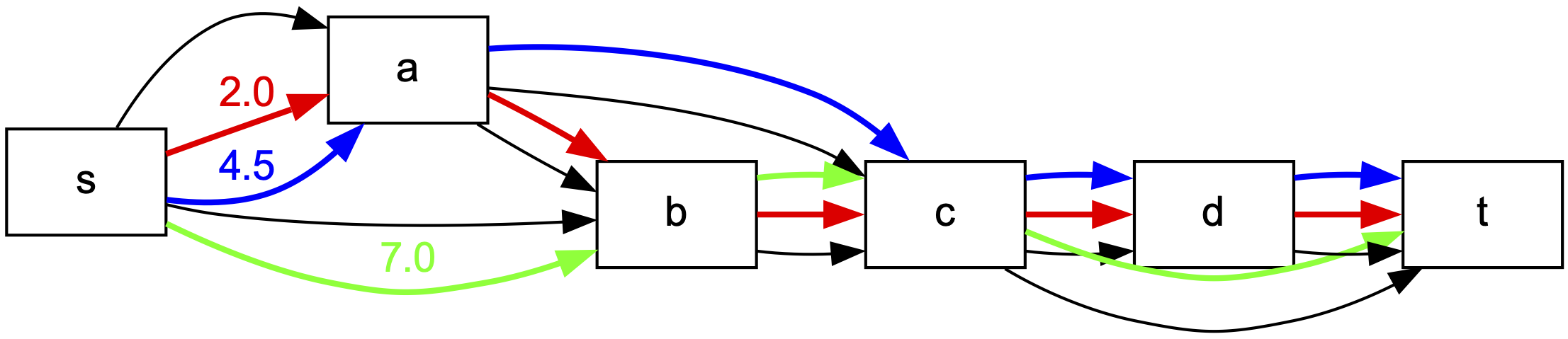
using the following code:
import flowpaths as fp
import networkx as nx

# Create a simple graph
graph = nx.DiGraph()
graph.graph["id"] = "simple_graph"
graph.add_edge("s", "a", flow=6)
graph.add_edge("s", "b", flow=7)
graph.add_edge("a", "b", flow=2)
graph.add_edge("a", "c", flow=5)
graph.add_edge("b", "c", flow=9)
graph.add_edge("c", "d", flow=6)
graph.add_edge("c", "t", flow=7)
graph.add_edge("d", "t", flow=6)

# Solve the minimum path error model
mpe_model = fp.kMinPathError(graph, flow_attr="flow", k=3, weight_type=float)
mpe_model.solve()

# Draw the solution
if mpe_model.is_solved():
    solution = mpe_model.get_solution()
    fp.utils.draw(
        G=graph,
        filename="simple_graph.pdf",
        flow_attr="flow",
        paths=solution["paths"],
        weights=solution["weights"],
        draw_options={
        "show_graph_edges": True,
        "show_edge_weights": False,
        "show_path_weights": False,
        "show_path_weight_on_first_edge": True,
        "pathwidth": 2,
    })
This produces a file with extension .pdf storing the PDF image of the graph.
Sankey Diagram Visualization
For acyclic graphs (DAGs), you can create interactive Sankey diagrams using plotly. Sankey diagrams are particularly effective for visualizing flow decompositions, as they show:
- Each node in the graph as a labeled box
- Each path as a colored flow whose width represents the path weight
To create a Sankey diagram, set "style": "sankey" in the draw_options:
import flowpaths as fp
import networkx as nx

# Create a sample DAG
G = nx.DiGraph()
G.add_edge('s', 'a', flow=10)
G.add_edge('s', 'b', flow=5)
G.add_edge('a', 'c', flow=6)
G.add_edge('a', 'd', flow=4)
G.add_edge('b', 'c', flow=3)
G.add_edge('b', 'd', flow=2)
G.add_edge('c', 't', flow=9)
G.add_edge('d', 't', flow=6)

# Compute minimum flow decomposition
solver = fp.MinFlowDecomp(G, flow_attr='flow')
solver.solve()
solution = solver.get_solution()

# Draw as interactive Sankey diagram
fp.utils.draw(
    G=G,
    filename="flow_sankey.html",  # saves as HTML (interactive)
    flow_attr='flow',
    paths=solution['paths'],
    weights=solution['weights'],
    draw_options={
        "style": "sankey"
    }
)
Features:
- Interactive: Hover over nodes and links to see details, zoom and pan the diagram
- Jupyter support: Automatically displays inline when run in Jupyter notebooks
- Dual output: Automatically saves both HTML (interactive) and a static image (PDF by default)
- Automatic coloring: Each path gets a distinct color; shared edges show blended colors
- Graph identification: Uses the graph’s ID as the diagram title if available
Requirements:
- plotly: Installed automatically with flowpaths
- kaleido: Installed automatically with flowpaths for static image export
File formats:
The function automatically saves both formats:
- HTML file (interactive): [basename].html
- Static image: [basename].pdf (or .png, .svg if specified)
# Saves both output.html and output.pdf
fp.utils.draw(G, "output", paths=paths, weights=weights,
              draw_options={"style": "sankey"})

# Saves both flow.html and flow.png
fp.utils.draw(G, "flow.png", paths=paths, weights=weights,
              draw_options={"style": "sankey"})

# Saves both diagram.html and diagram.svg
fp.utils.draw(G, "diagram.svg", paths=paths, weights=weights,
              draw_options={"style": "sankey"})
Note: Sankey diagrams require the graph to be acyclic (DAG). If the graph contains cycles, use the traditional graphviz rendering ("style": "default" or "style": "points").
See examples/sankey_demo.py and examples/sankey_demo.ipynb for complete examples.
Logging
flowpaths exposes a simple logging helper via fp.utils.configure_logging. Use it to control verbosity, enable console/file logging, and set file mode.
Basic usage (console logging at INFO level):
import flowpaths as fp

fp.utils.configure_logging(
    level=fp.utils.logging.INFO,
    log_to_console=True,
)
Also log to a file (append mode):
fp.utils.configure_logging(
    level=fp.utils.logging.DEBUG,      # default is DEBUG
    log_to_console=True,               # show logs in terminal
    log_file="flowpaths.log",         # write logs to this file
    file_mode="a",                    # "a" append (or "w" overwrite)
)
Notes:
- Levels available: fp.utils.logging.DEBUG, INFO, WARNING, ERROR, CRITICAL.
- Default level is DEBUG. If you prefer quieter output, use INFO or WARNING.
- Internally, the package logs through its own logger; configure_logging sets handlers/formatters accordingly.
API reference:
Configures logging for the flowpaths package.
Parameters:
-
level: int, optionalLogging level (e.g., fp.utils.logging.DEBUG, fp.utils.logging.INFO). Default is fp.utils.logging.DEBUG.
-
log_to_console: bool, optionalWhether to log to the console. Default is True.
-
log_file: str, optionalFile path to log to. If None, logging to a file is disabled. Default is None. If a file path is provided, the log will be written to that file. If the file already exists, it will be overwritten unless
file_modeis set to “a”. -
file_mode: str, optionalMode for the log file. “a” (append) or “w” (overwrite). Default is “w”.
Source code in flowpaths/utils/logging.py
check_flow_conservation
Check if the flow conservation property holds for the given graph.
Parameters
-
G: nx.DiGraphThe input directed acyclic graph, as networkx DiGraph.
-
flow_attr: strThe attribute name from where to get the flow values on the edges.
Returns
-
bool:
True if the flow conservation property holds, False otherwise.
Source code in flowpaths/utils/graphutils.py
draw
draw(
    G: DiGraph,
    filename: str,
    flow_attr: str = None,
    paths: list = [],
    weights: list = [],
    additional_starts: list = [],
    additional_ends: list = [],
    additional_edges: list = [],
    subpath_constraints: list = [],
    draw_options: dict = {
        "show_graph_edges": True,
        "show_edge_weights": False,
        "show_node_weights": False,
        "show_graph_title": False,
        "show_path_weights": False,
        "show_path_weight_on_first_edge": True,
        "pathwidth": 3.0,
        "style": "default",
        "color_nodes": False,
        "sankey_arrowlen": 0,
        "sankey_color_toggle": False,
        "sankey_arrow_toggle": False,
    },
)
Draw the graph with the paths and their weights highlighted.
Parameters
-
G: nx.DiGraphThe input directed acyclic graph, as networkx DiGraph.
-
filename: strThe name of the file to save the drawing. The file type is inferred from the extension. Supported extensions are ‘.bmp’, ‘.canon’, ‘.cgimage’, ‘.cmap’, ‘.cmapx’, ‘.cmapx_np’, ‘.dot’, ‘.dot_json’, ‘.eps’, ‘.exr’, ‘.fig’, ‘.gd’, ‘.gd2’, ‘.gif’, ‘.gtk’, ‘.gv’, ‘.ico’, ‘.imap’, ‘.imap_np’, ‘.ismap’, ‘.jp2’, ‘.jpe’, ‘.jpeg’, ‘.jpg’, ‘.json’, ‘.json0’, ‘.pct’, ‘.pdf’, ‘.pic’, ‘.pict’, ‘.plain’, ‘.plain-ext’, ‘.png’, ‘.pov’, ‘.ps’, ‘.ps2’, ‘.psd’, ‘.sgi’, ‘.svg’, ‘.svgz’, ‘.tga’, ‘.tif’, ‘.tiff’, ‘.tk’, ‘.vml’, ‘.vmlz’, ‘.vrml’, ‘.wbmp’, ‘.webp’, ‘.x11’, ‘.xdot’, ‘.xdot1.2’, ‘.xdot1.4’, ‘.xdot_json’, ‘.xlib’
-
flow_attr: strThe attribute name from where to get the flow values on the edges. Default is an empty string, in which case no edge weights are shown.
-
paths: listThe list of paths to highlight, as lists of nodes. Default is an empty list, in which case no path is drawn. Default is an empty list.
-
weights: listThe list of weights corresponding to the paths, of various colors. Default is an empty list, in which case no path is drawn.
-
additional_starts: listA list of additional nodes to highlight in green as starting nodes. Default is an empty list. -
additional_ends: listA list of additional nodes to highlight in red as ending nodes. Default is an empty list. -
additional_edges: listA list of additional edges to draw as dashed black lines if `show_graph_edges` is True. Each edge should be a tuple `(u, v)`. Default is an empty list. -
subpath_constraints: listA list of subpaths to highlight in the graph, of various colors. Each subpath can be:
- A list of nodes:
['n1', 'n2', 'n3', ...]— the nodes are highlighted with the constraint color, and edges between consecutive nodes are drawn as dashed lines. - A list of edges:
[('n1', 'n2'), ('n2', 'n3'), ...]— edges are drawn as dashed lines (existing behavior).
Default is an empty list. There is no association between the subpath colors and the path colors.
- A list of nodes:
-
draw_options: dictA dictionary with the following keys:
-
show_graph_edges: boolWhether to show the edges of the graph. Default is
True. -
show_edge_weights: boolWhether to show the edge weights in the graph from the
flow_attr. Default isFalse. -
show_node_weights: boolWhether to show the node weights in the graph from the
flow_attr. Default isFalse. -
show_graph_title: boolWhether to show the graph title (from graph id) in the figure. Default is
False. -
show_path_weights: boolWhether to show the path weights in the graph on every edge. Default is
False. -
show_path_weight_on_first_edge: boolWhether to show the path weight on the first edge of the path. Default is
True. -
pathwidth: floatThe width of the path to be drawn. Default is
3.0. -
style: strThe style of the drawing. Available options:
default,points,sankey.default: Standard graphviz rendering with nodes as rounded rectanglespoints: Graphviz rendering with nodes as pointssankey: Interactive Sankey diagram using plotly (requires acyclic graph). Saves as HTML by default (interactive) or static image formats (png, pdf, svg) if kaleido is installed. Automatically displays in Jupyter notebooks.
-
color_nodes: boolWhether to use the existing node coloring behavior. If `False` (default), all nodes use a neutral color. If `True`, nodes are colored as before (including `additional_starts` in green and `additional_ends` in red for graphviz styles). -
sankey_arrowlen: floatLength of arrowheads for Sankey links (Plotly
arrowlen). Default is0(no arrowheads). -
sankey_color_toggle: boolWhether to add an interactive toggle (buttons) to switch Sankey links between colored and monochrome gray. Default is
False. -
sankey_arrow_toggle: boolWhether to add an interactive toggle (buttons) to switch Sankey link arrowheads on/off. Default is
False.
-
Source code in flowpaths/utils/graphutils.py
787 788 789 790 791 792 793 794 795 796 797 798 799 800 801 802 803 804 805 806 807 808 809 810 811 812 813 814 815 816 817 818 819 820 821 822 823 824 825 826 827 828 829 830 831 832 833 834 835 836 837 838 839 840 841 842 843 844 845 846 847 848 849 850 851 852 853 854 855 856 857 858 859 860 861 862 863 864 865 866 867 868 869 870 871 872 873 874 875 876 877 878 879 880 881 882 883 884 885 886 887 888 889 890 891 892 893 894 895 896 897 898 899 900 901 902 903 904 905 906 907 908 909 910 911 912 913 914 915 916 917 918 919 920 921 922 923 924 925 926 927 928 929 930 931 932 933 934 935 936 937 938 939 940 941 942 943 944 945 946 947 948 949 950 951 952 953 954 955 956 957 958 959 960 961 962 963 964 965 966 967 968 969 970 971 972 973 974 975 976 977 978 979 980 981 982 983 984 985 986 987 988 989 990 991 992 993 994 995 996 997 998 999 1000 1001 1002 1003 1004 1005 1006 1007 1008 1009 1010 1011 1012 1013 1014 1015 1016 1017 1018 1019 1020 1021 1022 1023 1024 1025 1026 1027 1028 1029 1030 1031 1032 1033 1034 1035 1036 1037 1038 1039 1040 1041 1042 1043 1044 1045 1046 1047 1048 1049 1050 1051 1052 1053 1054 1055 1056 1057 1058 1059 1060 1061 1062 1063 1064 1065 1066 1067 1068 1069 1070 1071 1072 1073 1074 1075 1076 1077 1078 1079 1080 1081 1082 1083 1084 1085 1086 1087 1088 1089 1090 1091 1092 1093 1094 1095 1096 1097 1098 1099 1100 1101 1102 1103 1104 1105 1106 1107 1108 1109 1110 1111 1112 1113 1114 1115 1116 1117 1118 1119 1120 1121 1122 1123 1124 1125 1126 1127 1128 1129 1130 1131 1132 1133 1134 1135 1136 1137 1138 1139 1140 1141 1142 1143 1144 1145 1146 1147 1148 1149 1150 1151 1152 1153 1154 1155 1156 1157 1158 1159 1160 1161 1162 1163 1164 1165 1166 1167 1168 1169 1170 1171 1172 1173 1174 1175 1176 1177 1178 1179 1180 1181 1182 1183 1184 1185 1186 1187 1188 1189 1190 1191 1192 1193 1194 1195 1196 1197 1198 1199 1200 1201 1202 1203 1204 1205 1206 1207 1208 1209 1210 1211 1212 1213 1214 1215 1216 1217 1218 1219 1220 1221 1222 1223 1224 1225 1226 1227 1228 1229 1230 1231 1232 1233 1234 1235 1236 1237 1238 1239 1240 1241 1242 1243 1244 1245 1246 1247 1248 1249 1250 1251 1252 1253 1254 1255 1256 1257 1258 1259 1260 1261 1262 1263 1264 1265 1266 1267 1268 1269 1270 1271 1272 1273 1274 1275 1276 1277 1278 1279 1280 1281 1282 1283 1284 1285 1286 1287 1288 1289 1290 1291 1292 1293 1294 1295 1296 1297 1298 1299 1300 1301 1302 1303 1304 1305 1306 1307 1308 1309 1310 1311 1312 1313 1314 1315 1316 1317 1318 1319 1320 1321 1322 1323 1324 1325 1326 1327 1328 1329 1330 1331 1332 1333 1334 1335 1336 1337 | |
fpid
get_subgraph_between_topological_nodes
get_subgraph_between_topological_nodes(
    graph: DiGraph,
    topo_order: list,
    left: int,
    right: int,
) -> nx.DiGraph
Create a subgraph with the nodes between left and right in the topological order, including the edges between them, but also the edges from these nodes that are incident to nodes outside this range.
Source code in flowpaths/utils/graphutils.py
max_bottleneck_path
Computes the maximum bottleneck path in a directed graph.
Parameters
-
G: nx.DiGraphA directed graph where each edge has a flow attribute.
-
flow_attr: strThe flow attribute from where to get the flow values.
Returns
-
tuple: A tuple containing:
- The value of the maximum bottleneck.
- The path corresponding to the maximum bottleneck (list of nodes). If no s-t flow exists in the network, returns (None, None).
Source code in flowpaths/utils/graphutils.py
max_occurrence
Check what is the maximum number of edges of seq that appear in some path in the list paths_in_DAG.
This assumes paths_in_DAG are paths in a directed acyclic graph.
Parameters
- seq (list): The sequence of edges to check.
- paths (list): The list of paths to check against, as lists of nodes.
Returns
- int: the largest number of seq edges that appear in some path in paths_in_DAG
Source code in flowpaths/utils/graphutils.py
read_graph
Parse a single graph block from a list of lines.
Accepts one or more header lines at the beginning (each prefixed by ‘#’), followed by a line containing the number of vertices (n), then any number of edge lines of the form: “u v w” (whitespace-separated).
Subpath constraint lines
Lines starting with “#S” define a (directed) subpath constraint as a sequence of nodes: “#S n1 n2 n3 …”. For each such line we build the list of consecutive edge tuples [(n1,n2), (n2,n3), …] and append this edge-list (the subpath) to G.graph[“constraints”]. Duplicate filtering is applied on the whole node sequence: if an identical sequence of nodes has already appeared in a previous “#S” line, the entire subpath line is ignored (its edges are not added again). Different subpaths may
share edges; they are kept as separate entries. After all graph edges are parsed, every constraint edge is validated to ensure it exists in the graph; a missing edge raises ValueError.
Example block
graph number = 1 name = foo
any other header line
S a b c d (adds subpath [(a,b),(b,c),(c,d)])
S b c e (adds subpath [(b,c),(c,e)])
S a b c d (ignored: exact node sequence already seen)
5 a b 1.0 b c 2.5 c d 3.0 c e 4.0
Source code in flowpaths/utils/graphutils.py
258 259 260 261 262 263 264 265 266 267 268 269 270 271 272 273 274 275 276 277 278 279 280 281 282 283 284 285 286 287 288 289 290 291 292 293 294 295 296 297 298 299 300 301 302 303 304 305 306 307 308 309 310 311 312 313 314 315 316 317 318 319 320 321 322 323 324 325 326 327 328 329 330 331 332 333 334 335 336 337 338 339 340 341 342 343 344 345 346 347 348 349 350 351 352 353 354 355 356 357 358 359 360 361 362 363 364 365 366 367 368 369 370 371 372 373 374 375 | |
read_graphs
Read one or more graphs from a file.
Supports graphs whose header consists of one or multiple consecutive lines prefixed by ‘#’. Each graph block is: - one or more header lines starting with ‘#’ - one line with the number of vertices (n) - zero or more edge lines “u v w”
Graphs are delimited by the start of the next header (a line starting with ‘#’) or the end of file.
Source code in flowpaths/utils/graphutils.py
read_intron_graph
Read one node-weighted graph from a folder produced in the intron-graph TSV format.
Expected files inside graph_dir:
- vertices.tsv: node list. Each row becomes one graph node, with:
- node id from vertex_id
- node weight stored in G.nodes[node]["flow"] from the weight column
- extra metadata copied from the row (type, chr, start, end)
- edges.tsv: directed graph edges. The u and v columns define edges.
If a third weight column is present, it is stored on the edge as flow.
- read_subpaths.tsv (optional): subpath constraints. Each non-empty path_simple
value is parsed as a comma-separated node list and appended to
G.graph["constraints"].
- paths.tsv (optional): ground-truth transcript paths. For each row,
path_simple is parsed as a node list and stored in:
- G.graph["groundtruth_paths_nodes"] (list of node lists)
- G.graph["groundtruth_paths_edges"] (list of edge lists between consecutive nodes)
and count_scaled is stored in G.graph["groundtruth_weights"].
- ref_edges.tsv (optional): reference edge metadata. Rows with concrete
u_id, v_id values are collected in two groups:
- status == "in_graph" -> G.graph["reference_edges"]
- status == "missing_edge" -> G.graph["additional_edges"]
The returned graph uses node weights (flow) in the same spirit as read_ngraph.
It also stores:
- G.graph["id"]: folder name
- G.graph["source_folder"]: absolute folder path
- G.graph["constraints"]: list of node lists from read_subpaths.tsv:path_simple
- G.graph["groundtruth_paths_nodes"]: list of node lists from paths.tsv:path_simple
- G.graph["groundtruth_paths_edges"]: list of edge lists induced by groundtruth_paths_nodes
- G.graph["groundtruth_weights"]: list of count_scaled values from paths.tsv
- G.graph["reference_edges"]: list of in-graph (u_id, v_id) pairs from ref_edges.tsv
- G.graph["additional_edges"]: list of missing-edge (u_id, v_id) pairs from ref_edges.tsv
- G.graph["n"], G.graph["m"], G.graph["w"]: node count, edge count, width
Source code in flowpaths/utils/graphutils.py
34 35 36 37 38 39 40 41 42 43 44 45 46 47 48 49 50 51 52 53 54 55 56 57 58 59 60 61 62 63 64 65 66 67 68 69 70 71 72 73 74 75 76 77 78 79 80 81 82 83 84 85 86 87 88 89 90 91 92 93 94 95 96 97 98 99 100 101 102 103 104 105 106 107 108 109 110 111 112 113 114 115 116 117 118 119 120 121 122 123 124 125 126 127 128 129 130 131 132 133 134 135 136 137 138 139 140 141 142 143 144 145 146 147 148 149 150 151 152 153 154 155 156 157 158 159 160 161 162 163 164 165 166 167 168 169 170 171 172 173 174 175 176 177 178 179 180 181 182 183 184 185 186 187 188 189 190 191 192 193 194 195 196 197 198 199 200 201 202 203 204 205 206 207 208 209 210 211 212 213 214 215 216 217 218 219 220 221 | |
read_intron_graphs
Read all intron-format graph folders inside foldername.
Behavior:
- If foldername itself contains vertices.tsv, it is parsed as one graph folder.
- Otherwise, every immediate child directory containing vertices.tsv is parsed.
Returns a list of graphs in lexicographic folder-name order.
Source code in flowpaths/utils/graphutils.py
read_ngraph
Parse a single node-weighted ngraph block from a list of lines.
Expected block structure
- one or more leading header lines starting with ‘#’ (optional #S constraints can appear here)
- one line with the number of nodes n
- a marker line starting with ‘#NODES’
- exactly n node lines: “node_id node_weight”
- a marker line starting with ‘#EDGES’
- zero or more edge lines: “u v edge_weight”
Constraint lines
- ‘#S n1 n2 n3 …’ lines define subpath constraints.
- Duplicates are filtered by exact node sequence.
- Constraints are stored in G.graph[‘constraints’] as node lists.
Source code in flowpaths/utils/graphutils.py
423 424 425 426 427 428 429 430 431 432 433 434 435 436 437 438 439 440 441 442 443 444 445 446 447 448 449 450 451 452 453 454 455 456 457 458 459 460 461 462 463 464 465 466 467 468 469 470 471 472 473 474 475 476 477 478 479 480 481 482 483 484 485 486 487 488 489 490 491 492 493 494 495 496 497 498 499 500 501 502 503 504 505 506 507 508 509 510 511 512 513 514 515 516 517 518 519 520 521 522 523 524 525 526 527 528 529 530 531 532 533 534 535 536 537 538 539 540 541 542 543 544 545 546 547 548 549 550 551 552 553 554 555 556 557 558 559 560 561 562 563 564 565 566 567 568 569 570 571 572 573 574 575 576 577 578 579 580 581 582 583 584 585 | |
read_ngraphs
Read one or more ngraph blocks from a file.
Graph blocks are delimited by lines starting with ‘# graph’ (case-insensitive). If no such delimiter exists, the whole file is parsed as one ngraph block.